Theoretical PC energy of deep linear networks¤
![]()
This notebook demonstrates how to compute the theoretical PC energy at the inference equilibrium \(\mathcal{F}^*\) when \(\nabla_{\mathbf{z}} \mathcal{F} = \mathbf{0}\) for deep linear networks (Innocenti et al., 2024). For a set of inputs and outputs \(\{(\mathbf{x}_i, \mathbf{y}_i)\}_{i=1}^N\), this is given by
where \(\mathbf{S} = \mathbf{I}_{d_y} + \sum_{\ell=2}^L (\mathbf{W}_{L:\ell})(\mathbf{W}_{L:\ell})^T\) and \(\mathbf{W}_{k:\ell} = \mathbf{W}_k \dots \mathbf{W}_\ell\) for \(\ell, k \in 1,\dots, L\). This result can be generalised to any linear layer transformation \(\mathbf{B}_\ell\), e.g. for a ResNet \(\mathbf{B}_\ell = \mathbf{I} + \mathbf{W}_\ell\) (see Innocenti et al., 2025).
%%capture
!pip install torch==2.3.1
!pip install torchvision==0.18.1
!pip install plotly==5.11.0
!pip install -U kaleido
import jpc

import jax
import jax.numpy as jnp
import equinox as eqx
import optax

import torch
from torch.utils.data import DataLoader
from torchvision import datasets, transforms

import matplotlib.pyplot as plt

import warnings
warnings.simplefilter('ignore')  # ignore warnings
Hyperparameters¤
We define some global parameters, including the network architecture, learning rate, batch size, etc.
SEED = 0

INPUT_DIM = 784
WIDTH = 300
DEPTH = 5
OUTPUT_DIM = 10
ACT_FN = "linear"

LEARNING_RATE = 1e-3
BATCH_SIZE = 64
MAX_T1 = 300
TEST_EVERY = 10
N_TRAIN_ITERS = 100
Dataset¤
Some utils to fetch MNIST.
def get_mnist_loaders(batch_size):
    train_data = MNIST(train=True, normalise=True)
    test_data = MNIST(train=False, normalise=True)
    train_loader = DataLoader(
        dataset=train_data,
        batch_size=batch_size,
        shuffle=True,
        drop_last=True
    )
    test_loader = DataLoader(
        dataset=test_data,
        batch_size=batch_size,
        shuffle=True,
        drop_last=True
    )
    return train_loader, test_loader


class MNIST(datasets.MNIST):
    def __init__(self, train, normalise=True, save_dir="data"):
        if normalise:
            transform = transforms.Compose(
                [
                    transforms.ToTensor(),
                    transforms.Normalize(
                        mean=(0.1307), std=(0.3081)
                    )
                ]
            )
        else:
            transform = transforms.Compose([transforms.ToTensor()])
        super().__init__(save_dir, download=True, train=train, transform=transform)

    def __getitem__(self, index):
        img, label = super().__getitem__(index)
        img = torch.flatten(img)
        label = one_hot(label)
        return img, label


def one_hot(labels, n_classes=10):
    arr = torch.eye(n_classes)
    return arr[labels]
Plotting¤
def plot_total_energies(energies):
    n_train_iters = len(energies["theory"])
    train_iters = [b+1 for b in range(n_train_iters)]

    _, ax = plt.subplots(figsize=(6, 3))

    for energy_type, energy in energies.items():
        is_theory = energy_type == "theory"
        line_style = "--" if is_theory else "-"
        color = "black" if is_theory else "#00CC96"  #"rgb(27, 158, 119)"

        if color.startswith("rgb"):
            rgb = tuple(int(x)/255 for x in color[4:-1].split(","))
        else:
            rgb = color

        ax.plot(
            train_iters,
            energy,
            label=energy_type,
            linewidth=3 if is_theory else 2,
            linestyle=line_style,
            color=rgb
        )

    ax.legend(fontsize=16)
    ax.set_xlabel("Training Iteration", fontsize=18, labelpad=10)
    ax.set_ylabel("Energy", fontsize=18, labelpad=10)
    ax.tick_params(axis='both', labelsize=14)
    plt.grid(True)
    plt.show()
Train and test¤
To compute the theoretical energy, we can use jpc.linear_equilib_energy() which as clear from the equation above just takes a linear network and some data.
def evaluate(model, test_loader):
    avg_test_loss, avg_test_acc = 0, 0
    for _, (img_batch, label_batch) in enumerate(test_loader):
        img_batch, label_batch = img_batch.numpy(), label_batch.numpy()

        test_loss, test_acc = jpc.test_discriminative_pc(
            model=model,
            output=label_batch,
            input=img_batch
        )
        avg_test_loss += test_loss
        avg_test_acc += test_acc

    return avg_test_loss / len(test_loader), avg_test_acc / len(test_loader)


def train(
      input_dim,
      width,
      depth,
      output_dim,
      act_fn,
      lr,
      batch_size,
      max_t1,
      test_every,
      n_train_iters
):
    key = jax.random.PRNGKey(0)

    # NOTE: act_fn is linear and we use no biases
    model = jpc.make_mlp(
        key,
        input_dim=input_dim,
        width=width,
        depth=depth,
        output_dim=output_dim,
        act_fn=act_fn,
        use_bias=False
    )
    optim = optax.adam(lr)
    opt_state = optim.init(
        (eqx.filter(model, eqx.is_array), None)
    )
    train_loader, test_loader = get_mnist_loaders(batch_size)

    num_total_energies, theory_total_energies = [], []
    for iter, (img_batch, label_batch) in enumerate(train_loader):
        img_batch, label_batch = img_batch.numpy(), label_batch.numpy()

        theory_total_energies.append(
            jpc.linear_equilib_energy(
                params=(model, None),
                x=img_batch,
                y=label_batch
            )
        )
        result = jpc.make_pc_step(
            model,
            optim,
            opt_state,
            output=label_batch,
            input=img_batch,
            max_t1=max_t1,
            record_energies=True
        )
        model, opt_state = result["model"], result["opt_state"]
        train_loss, t_max = result["loss"], result["t_max"]
        num_total_energies.append(result["energies"][:, t_max-1].sum())

        if ((iter+1) % test_every) == 0:
            _, avg_test_acc = evaluate(model, test_loader)
            print(
                f"Train iter {iter+1}, train loss={train_loss:4f}, "
                f"avg test accuracy={avg_test_acc:4f}"
            )
            if (iter+1) >= n_train_iters:
                break

    return {
        "theory": jnp.array(theory_total_energies),
        "experiment": jnp.array(num_total_energies)
    }
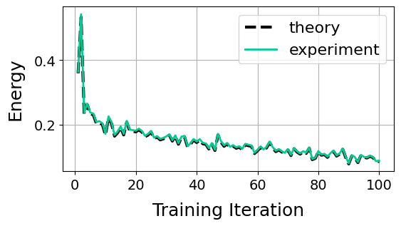
Run¤
Below we plot the theoretical energy against the numerical one.
energies = train(
    input_dim=INPUT_DIM,
    width=WIDTH,
    depth=DEPTH,
    output_dim=OUTPUT_DIM,
    act_fn=ACT_FN,
    lr=LEARNING_RATE,
    batch_size=BATCH_SIZE,
    test_every=TEST_EVERY,
    max_t1=MAX_T1,
    n_train_iters=N_TRAIN_ITERS
)
plot_total_energies(energies)
Train iter 10, train loss=0.267786, avg test accuracy=72.786461
Train iter 20, train loss=0.288985, avg test accuracy=75.811295
Train iter 30, train loss=0.271584, avg test accuracy=79.156654
Train iter 40, train loss=0.253959, avg test accuracy=81.951118
Train iter 50, train loss=0.262732, avg test accuracy=81.079727
Train iter 60, train loss=0.237084, avg test accuracy=80.398636
Train iter 70, train loss=0.259781, avg test accuracy=80.889420
Train iter 80, train loss=0.264378, avg test accuracy=82.091347
Train iter 90, train loss=0.193282, avg test accuracy=82.251602
Train iter 100, train loss=0.230495, avg test accuracy=80.298477