Unsupervised generative PC¤
![]()
This notebook demonstrates how to train a simple feedforward network with predictive coding to encode MNIST digits in an unsupervised manner.
import jpc

import jax
import equinox as eqx
import equinox.nn as nn
import optax

import torch
from torch.utils.data import DataLoader
from torchvision import datasets, transforms

import matplotlib.pyplot as plt
import matplotlib.colors as mcolors

import warnings
warnings.simplefilter('ignore')  # ignore warnings
Hyperparameters¤
We define some global parameters, including the network architecture, learning rate, batch size, etc.
SEED = 0

INPUT_DIM = 50
WIDTH = 300
DEPTH = 3
OUTPUT_DIM = 784
ACT_FN = "relu"

LEARNING_RATE = 1e-3
BATCH_SIZE = 64
MAX_T1 = 100
N_TRAIN_ITERS = 300
Dataset¤
Some utils to fetch and plot MNIST.
def get_mnist_loaders(batch_size):
    train_data = MNIST(train=True, normalise=True)
    test_data = MNIST(train=False, normalise=True)
    train_loader = DataLoader(
        dataset=train_data,
        batch_size=batch_size,
        shuffle=True,
        drop_last=True
    )
    test_loader = DataLoader(
        dataset=test_data,
        batch_size=batch_size,
        shuffle=True,
        drop_last=True
    )
    return train_loader, test_loader


class MNIST(datasets.MNIST):
    def __init__(self, train, normalise=True, save_dir="data"):
        if normalise:
            transform = transforms.Compose(
                [
                    transforms.ToTensor(),
                    transforms.Normalize(
                        mean=(0.1307), std=(0.3081)
                    )
                ]
            )
        else:
            transform = transforms.Compose([transforms.ToTensor()])
        super().__init__(save_dir, download=True, train=train, transform=transform)

    def __getitem__(self, index):
        img, _ = super().__getitem__(index)
        img = torch.flatten(img)
        return img
Plotting¤
def plot_train_energies(energies, ts):
    t_max = int(ts[0])
    norm = mcolors.Normalize(vmin=0, vmax=len(energies)-1)
    fig, ax = plt.subplots(figsize=(8, 4))

    cmap_blues = plt.get_cmap("Blues")
    cmap_reds = plt.get_cmap("Reds")
    cmap_greens = plt.get_cmap("Greens")

    legend_handles = []
    legend_labels = []

    for t, energies_iter in enumerate(energies):
        line1, = ax.plot(energies_iter[0, :t_max], color=cmap_blues(norm(t)))
        line2, = ax.plot(energies_iter[1, :t_max], color=cmap_reds(norm(t)))
        line3, = ax.plot(energies_iter[2, :t_max], color=cmap_greens(norm(t)))

        if t == 70:
            legend_handles.append(line1)
            legend_labels.append("$\ell_1$")
            legend_handles.append(line2)
            legend_labels.append("$\ell_2$")
            legend_handles.append(line3)
            legend_labels.append("$\ell_3$")

    ax.legend(legend_handles, legend_labels, loc="best", fontsize=16)
    sm = plt.cm.ScalarMappable(cmap=plt.get_cmap("Greys"), norm=norm)
    sm._A = []
    cbar = fig.colorbar(sm, ax=ax)
    cbar.set_label("Training iteration", fontsize=16, labelpad=14)
    cbar.ax.tick_params(labelsize=14)
    plt.gca().tick_params(axis="both", which="major", labelsize=16)

    ax.set_xlabel("Inference iterations", fontsize=18, labelpad=14)
    ax.set_ylabel("Energy", fontsize=18, labelpad=14)
    ax.set_yscale("log")
    plt.show()
Network¤
For jpc to work, we need to provide a network with callable layers. This is easy to do with the PyTorch-like nn.Sequential() in equinox. For example, we can define a ReLU MLP with two hidden layers as follows
key = jax.random.PRNGKey(SEED)
key, *subkeys = jax.random.split(key, 4)
network = [
    nn.Sequential(
        [
            nn.Linear(10, 300, key=subkeys[0]),
            nn.Lambda(jax.nn.relu)
        ],
    ),
    nn.Sequential(
        [
            nn.Linear(300, 300, key=subkeys[1]),
            nn.Lambda(jax.nn.relu)
        ],
    ),
    nn.Linear(300, 784, key=subkeys[2]),
]
You can also use jpc.make_mlp() to define a multi-layer perceptron (MLP) or fully connected network.
network = jpc.make_mlp(
    key,
    input_dim=INPUT_DIM,
    width=WIDTH,
    depth=DEPTH,
    output_dim=OUTPUT_DIM,
    act_fn=ACT_FN,
    use_bias=True
)
print(network)
[Sequential(
  layers=(
    Lambda(fn=Identity()),
    Linear(
      weight=f32[300,50],
      bias=f32[300],
      in_features=50,
      out_features=300,
      use_bias=True
    )
  )
), Sequential(
  layers=(
    Lambda(fn=<PjitFunction of <function relu at 0x12db01e10>>),
    Linear(
      weight=f32[300,300],
      bias=f32[300],
      in_features=300,
      out_features=300,
      use_bias=True
    )
  )
), Sequential(
  layers=(
    Lambda(fn=<PjitFunction of <function relu at 0x12db01e10>>),
    Linear(
      weight=f32[784,300],
      bias=f32[784],
      in_features=300,
      out_features=784,
      use_bias=True
    )
  )
)]
Train¤
A PC network can be updated in a single line of code with jpc.make_pc_step(), which is already "jitted" for optimised performance. To train in an unsupervised way, we simply avoid providing an input to jpc.make_pc_step(). To test the learned encoding or representation for downstream accuracy, you could simply add a classifier.
def train(
      key,
      input_dim,
      width,
      depth,
      output_dim,
      batch_size,
      network,
      lr,
      max_t1,
      n_train_iters
):
    layer_sizes = [input_dim] + [width]*(depth-1) + [output_dim]
    optim = optax.adam(lr)
    opt_state = optim.init(
        (eqx.filter(network, eqx.is_array), None)
    )
    train_loader, _ = get_mnist_loaders(batch_size)

    train_energies, ts = [], []
    for iter, img_batch in enumerate(train_loader):
        img_batch = img_batch.numpy()

        result = jpc.make_pc_step(
            key=key,
            layer_sizes=layer_sizes,
            batch_size=batch_size,
            model=network,
            optim=optim,
            opt_state=opt_state,
            output=img_batch,
            max_t1=max_t1,
            record_activities=True,
            record_energies=True
        )
        network, opt_state = result["model"], result["opt_state"]
        train_energies.append(result["energies"])
        ts.append(result["t_max"])
        if (iter+1) >= n_train_iters:
            break

    return result["model"], train_energies, ts
Run¤
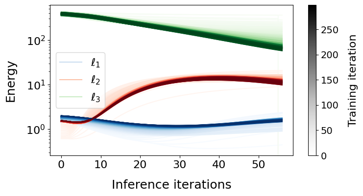
Below we simply plot the energy dynamics of each layer during both inference and learning.
network, energies, ts = train(
    key=key,
    input_dim=INPUT_DIM,
    width=WIDTH,
    depth=DEPTH,
    output_dim=OUTPUT_DIM,
    batch_size=BATCH_SIZE,
    network=network,
    lr=LEARNING_RATE,
    max_t1=MAX_T1,
    n_train_iters=N_TRAIN_ITERS
)
plot_train_energies(energies, ts)